DQN to play Space Invaders
Introduction
When we think about the nature of learning, and how humans and animals discover the structure of the world, we find that it is more like a trial-and-error process than anything else. In fact, we are not being told how to act or what to do at each situation in our life, but instead we learn by observing and trying things out to see what the outcome will be.
When a toddler learns how to walk, his objective is to stay upright, in such case he is going to get a hug from his parents who are happy that their toddler has successfully taken his first steps (positive reward), and avoid falling down, in such case, his legs are going to be harmed (negative reward). Based on this continuous interaction between the toddler and his environment, he adjusts his behavior based on the feedback he receives; in this case a hug or harming his legs, each time he tries an action. And by doing so, he ends up learning how to walk.
The core of Reinforcement Learning (RL) is based on the concept that the optimal behavior is reinforced by a positive reward. Just like the teetering toddler, a robot that is learning to walk with RL will try different ways to achieve the objective, gets feedback about how successful those ways were, and then adjusts his behavior until the aim to walk is achieved. A big step forward makes the robot fall, so it adjusts its step to make it smaller in order to see if that is the secret to staying upright. By doing so, optimal actions yielding a positive reward get reinforced, and ultimately the robot is able to walk.
Nowadays, RL techniques have proven themselves powerful in a large spectrum of applications and are to be found everywhere the decision making process is sequential. Still, the ideal testbed for these methods and algorithms are video games. They provide a virtual environment in which an agent is thrown to figure its way out while maximizing the score of the game, just as its counterpart human player do.
A few years ago, Deepmind released the Deep Q Network (DQN) architecture that demonstrated its ability to master Atari 2600 computer games, using only raw pixels as input. In this post I thought it would be fun to experiment with this architecture by playing Space Invaders. I’ll start by laying out the mathematics of RL before moving on to describe the DQN architecture and its application to our specific game. Lastly, I will go through some implementation details, whose code is available on my Github repository.
A brief overview with links to the relevant sections is given below:
$\text{I}$ - Background.
$\text{II}$ - Mathematics behind RL.
$\text{III}$ - Implementation details.
$\text{IV}$ - Results.
$\text{V}$ - Conclusion
$\text{VI}$ - Resources and further reading
$\text{I}$ - Background
$\text{I.1}$ - What is RL ?
Reinforcement learning is a subfield of machine learning and a stochastic dynamic programming approach that concentrates on the concept of trial-and- error learning through the interaction between two major entities, that are a decision-maker called the agent and a dynamic environment, via their communication channels, that are the state, action and reward.
The state summarizes the information the agent senses from the environment at each time step $t$, while the action is the decision the agent has to make in order to receive a numerical reward as a feedback from the environment assessing the goodness or badness of the decision that has been made.
This approach generally consists of cycles, in which the environment is at a given state, and the agent should take an action, dictated by a policy — which is a function mapping from the environment state space to the environment action space — that will be evaluated later by the environment which sends a feedback, in the form of a numerical reward, on the decision that has been made, as depicted in Figure 1. While the environment’s state changes thereafter, the agent tries to improve its behavior, i.e. policy, based on the reward he had received, and a new cycle starts again.
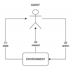
Figure 1: Environment-Agent interface. (Drawn using draw.io)
$\text{I.2}$ - Why RL ?
Because RL models learn by a continuous process of receiving rewards and punishments on every action taken, they are able to train themselves to respond to unforeseen environments. RL is ideal when we know what we want a system to do, but are unable to take into account all the possible scenarios of a specific process by hard-coding them and/or the list of potential random hazards within the system is embarrassingly large. Concretely, we create a simulation of our problem, and let the artificial agent learns the optimal way to behave in this simulation. Eventually, we pick this optimal behavior and plug it into our original problem.
$\text{II}$ - Mathematics behind RL
$\text{II.1}$ - Modeling the environment
The environment is modeled using a Markov Decision Process (MDP), which is a tuple $(S, A, P, R, \gamma)$, where:
-
$S$ is a finite set of states.
-
$A$ is a finite set of actions.
-
$P$ is a transition matrix :
-
$R$ is a reward function :
\[R^{s}_{a}=E[R_{t+1}|S_t=s, A_t=a]\] -
$\gamma$ is a discount factor lying within the interval $]0, 1]$.
The transition $P$ and the reward function $R$ are referred to in the literature as the model of the environment. For the purpose of this post, we are not going to implement the environment from scratch. Instead, we are going to use OpenAI gym. It is an easy to use open-source library used for evaluating, and comparing RL algorithms on plethora of built-in environments. It is compatible with any deep learning framework such as PyTorch, TensorFlow, Theano, etc.. Also, it makes no assumption about the structure of the agent. Thus, it provides this flexibility to design the agent based on any paradigm the user chooses. For the purpose of this post, we are going to work with the Space Invaders’ environment.
$\text{II.2}$ - Reward vs Return
As discussed earlier, RL agents interact with the environment to collect information and experience which it will then use to train itself and update its behavior in order to get more and more rewards in the future. The immediate feedback the agent gets from the environment is called reward $R_t$, whereas the cumulative future reward the agent has to maximize is called the return, and is denoted $G_t$ at each time step $t$. The relationship between the two is the following:
\[G_t = \sum_{0\leq k \leq \inf} \gamma^k R_{t+k}\]Note the use of the discount factor $\gamma$ to show preference for the immediate rewards and also to get the series $G_t$ to converge in the case of infinite games. The return is what drives the agent to find its way in a given environment.
$\text{II.3}$ - Modeling the agent
The agent is modeled using a Deep Q Network (DQN), which is a variant of the Q-Learning algorithm. But before we get into DQNs, we have to introduce some new concepts as well as some useful notations.
$\text{II.3.a}$ - Policy $\pi$
A policy function $\pi$, is a mapping from the environment set of states $S$ to the environment set of actions $A$. Two classes of policies can be distinguished:
-
Deterministic policy: is a deterministic mapping: $\pi: S \rightarrow A$ that assigns to each state some fixed action. For example:
Let $S={s_1, s_2}$ be the state space and $A={a_1, a_2}$ be the the action space. An example of a deterministic policy can be defined as:
\[\pi(s_1)=a_1\] \[\pi(s_2)=a_2\]which means that whenever the agent is in state $s_1$, it will choose action $a_1$ and whenever in state $s_2$ it will choose action $a_2$.
-
Stochastic policy: is a probability distribution over the set of actions given a particular state of the environment. If we take the last example, a stochastic policy can be defined as follows:
\[\pi(a_1|s_1)=0.8; \pi(a_2|s_1)=0.2\]
This means that whenever the agent is in the state $s_1$, it will take the action $a_1$ or $a_2$ with probability of $0.8$ and $0.2$ respectively, and whenever it is in the state $s_2$, it will take the action $a_1$ with probability $0.3$ and action $a_2$ with probability $0.7$.
In a nutshell, the agent’s aim is to learn the optimal policy, denoted \(\pi^*\) that has the property of yielding actions that maximizes the cumulative reward \(G_t\) in the long run. One way for the agent to compare between policies when learning is to use an action-value function.
$\text{II.3.b}$ - Action-Value function $Q^{\pi}$
$Q^{\pi}$ answers the question of how good it is for the agent to take action $a$ in state $s$ while following policy $\pi$. It is a function mapping a state $s \in S$ and an action $a \in A$ to the discounted return $G_t$ the agent can expect to get after making this move. Mathematically, $Q^{\pi}$ is defined as follows:
\[Q^{\pi}(s, a) = \text{E}_{\pi}[G_t|S_t=s, A_t=a]\]The expectation takes into account the randomness in future actions according to the policy, as well as the randomness of the returned rewards from the environment.
Note that $Q^\pi$ depends on the policy $\pi$. Thus, for the same environment, the action-value function may change depending on the policy the agent is using to get his actions. To better grasp this point, we can rewrite $Eq.\ 6$ by introducing $\pi$ in the right hand-side of the equation:
\[Q^{\pi}(s, a) = \text{E}_{\pi}[G_t|S_t=s, A_t=\pi(s)]\]$\text{II.3.c}$ - Expressing $Q^{\pi}$ recursively: Bellman’s Equation
I won’t go through a step-by-step derivation (though you can find one here and another one here), but by just using the definition of $Q^\pi$ and $G_t$ as well as some algebra, we can show that $Q^{\pi}$ can be written recursively:
\[Q^{\pi}(s, a) = \text{E}_{\pi}[R_{t} + \gamma Q^{\pi}(S_{t+1}, A_{t+1})|S_t=s, A_t=a]\]What this recursive expression, called the Bellman’s Equation, says is that an action from a state is good if it either gives you a high reward or it leads you to a state in which actions to be taken are good. The importance of the Bellman’s Equation is that it let us express values of states as a function of values of their successors. This opens the door to lots of iterative approaches for numerically calculating the action-value function. Finally, note that the Bellman’s Equation is deduced purely from the very definition of the $Q$ function. This means that for an arbitrary function to be a valid $Q$ function, it must satisfy the Bellman’s Equation. This is a crucial note to remember that will help us later when implementing DQN.
If the agent keeps updating its $Q$ function, it converges eventually to the optimal $Q$ function, denoted $Q^*$:
\[Q^{*}(s, a) = \text{max}_{\pi}Q^{\pi}(s, a)\]$\text{II.3.d}$ - Optimality equations: \(\pi^*\) and \(Q^{*}\)
The RL agent seeks to find the policy $\pi$ that yields more return than any other policy. This policy is called the optimal policy, denoted \(\pi^*\). This is a lookup in the space \(\Pi\) of all possible policies for a policy that satisfies the following statement:
\[\text{ for each state } s \in S, \text{ for each action } a \text{ out of } s, \ \pi \geq \pi' \text{ if and only if } Q^\pi(s, a) \geq Q^{\pi'}(s, a)\]In $Q$-Learning; the class of RL algorithms to which DQN belongs, we don’t optimize over \(\Pi\) directly to find \(\pi^*\). Instead, we start by finding the optimal action-value function \(Q^*\) and the optimal policy easily follows. The later can be extracted by choosing the action $a$ that gives the greatest \(Q^*(s, a)\) for a given state $s$:
\[\pi^*(s)=arg\ max_a Q^*(s, a) \ \forall s \in S\]It turns out that finding \(Q^*\) is a pretty straightforward job if we follow Bellman’s Equation. In fact, we can show that \(Q^*(s, a)\) satisfies the so-called Bellman Optimality Equation: (full proof to be found here)
\[Q^*(s, a)=\text{E}[R_{t} + \gamma \max_{a'}{Q^{*}(s', a')}]\]where $s’$ is the successor state of $s$ and $a’$ is each of the actions out of $s’$.
To sum up, $\text{Eq.}\ 12$ is at the heart of $Q$-Learning. The whole purpose of $Q$-Learning is to learn the optimal $Q$-function. Once we have \(Q^*\), we use $\text{Eq.}\ 11$ to derive the optimal policy \(\pi^*\). And at this point, you can safely say that you had solved your environment !
$\text{II.4}$ - Q-Learning in a nutshell
Tabular $Q$-Learning is a primitive version of DQN. The idea behind it is to iteratively updating $Q$-values using the Bellman optimality equation ($Eq.\ 15$) until converging to $Q^{*}$. This approach is called Value-Iteration.
Consider the example, depicted in Figure 2, of an environment, modeled as an MDP, where we have a state space $S={s_1, s_2, s_3}$, with $s_3$ being the terminal or absorbing state in which the episode ends. Each arrow out of each state corresponds to a possible action $a_{ij}$ that takes the agent from one state to another. Finally, each action in each state is associated with a particular reward $R_{ij}$.
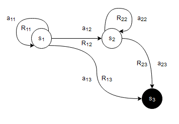
Figure 2: Example of an MDP. (Drawn using draw.io)
The agent makes use of the table below, called a $Q$-table, where it stores $Q$-values of each pair $(s, a)$, for each possible state $s \in S$ and for each possible action $a$ out of $s$.
| possible states | possible actions out of each state | action-value function |
|---|---|---|
| $s_1$ | $a_{11}$ | $Q(s_1, a_{11})$ |
| $s_1$ | $a_{12}$ | $Q(s_1, a_{12})$ |
| $s_1$ | $a_{13}$ | $Q(s_1, a_{13})$ |
| $s_2$ | $a_{21}$ | $Q(s_2, a_{21})$ |
| $s_2$ | $a_{22}$ | $Q(s_2, a_{22})$ |
Concretely, the agent starts by initializing the $Q$-values for each state-action pairs to zero, since it has no knowledge yet about the environment nor the expected rewards it can get for a given state-action pair. Throughout the game, though, it will update its $Q$-table using rewards it gathers from its interactions with the environment. More specifically, whenever the agent is in a given state $s$, it will refer to its $Q$-table to choose the best action $a$ out of $s$; the best action $a$ being the one that has the highest $Q$-value $Q(s, a)$. After taking this particular action in this particular state and receiving a reward from the environment, the agent will use this information to update its knowledge about the $Q$-value associated with this particular state-action pair, using the Bellman optimality equation ($Eq.\ 15$). As the training progresses and as the agent plays several episodes, it hopefully gets the chance to visit each state-action pair so that each $Q$-value in the $Q$-table get the chance to be updated. By the end of training, the $Q$-table ends up converging to $Q^*$.
$\text{II.5}$ - DQN as a combination of tabular Q-Learning and neural networks
By now, I think you already have noticed the limitations of tabular $Q$-Learning. More specifically, imagine a problem where we have an infinite number of states and an infinite number of actions out of each state. Keeping track of all the possible $Q$-values by storing them in a table is unfeasible and computationally intractable. One solution for extending tabular $Q$-learning to richer environments is to apply function approximators that take states and actions as inputs to learn the $Q$-function. Speaking of function approximators, neural networks to the rescue as the universal function approximators. The table I have drawn earlier is similar to a dataset in the supervised learning setting, where we have an input vector $X$ and want to predict a target value $y$. In the case of $Q$-Learning, the input vector is the state-action pairs, whereas the target is the action-value function $Q(s, a)$. Thus, we simply want to learn a mapping $ S \times A \rightarrow R $. Therefore our problem can easily be modeled as a supervised learning problem.
$\text{II.5.a}$ - Training a DQN
The agent constructs its own set of training data by playing several episodes of the game, starting with zero knowledge of the latter. At first, it plays poorly, but progressively, as it gathers more experience and collects more data, the quality of the training set improves. The technique that is used in training is called experience replay. It consists of maintaining a replay buffer, which is a set of all previous sequences that have been experienced. The goal is to build a training dataset from which we randomly sample several batches later when we will need to train the agent.
The reasons for building such buffer are: 1) gradient descent, which is the optimization algorithm used to update the networks’ parameters, works best with identically and independently distributed (i.i.d) samples. If we were to train the agent as it is collecting experience, also called online learning, there would be a strong temporal and chronological correlation between the samples, which compromises the learning and make it unstable. 2) if we do not use a buffer to store experiences, then a sequence is used only once and discarded afterwards, which may result in losing valuable information over time.
However, in practice, we want to keep the replay buffer as fresh as possible. Thus, the most suitable data structure that can be used is a deque with a maximum storage limit. This allows the agent to keep track only of recent sequences and discard the very old ones that were stored back when the agent had a less trained policy.
$\text{II.5.b}$ - DQN loss function
We said earlier that for an arbitrary function to be considered a valid action-value function, it must necessary satisfy the Bellman’s Equation. We can set up a mean-squared Bellman error (MSBE) function, which tells us roughly how closely the DQN $Q_w$ comes to satisfying the Bellman’s Equation, using a batch of samples sampled from the replay buffer:
\[L(Q_w)=\frac{1}{N}\sum_i(y_i-Q_w(s_i, a_i))^2\]where:
- $N$ is the batch size
- $y_i$ is called the TD target (right hand-side of the Bellman’s Equation) and is given by:
- where $s_{i+1}$ is the successor state of \(s_{i}\).
The quantity \(\delta_i= y_i-Q_w(s_i, a_i)\) is referred to in the literature as the TD error.
$\text{III}$ - Implementation details
The task we are concerned about is learning to play the popular Atari game Space Invaders. As it is the case in any game, the player’s goal is to maximize his score. To achieve this goal, the player must be able to refine its decision-making abilities. When he observes the state of the game at a given time, he must be able to pick an action, hopefully the best action, given the state of the game. In our case, the player is a DQN agent. Its decision-making process is governed by the policy, that accepts a state of the game as input and returns or “decides” on the best action to take.
Formally, the Space Invaders game play is discretized into time-steps running in an emulator. At each time step $t$, the emulator sends the state of the game $S_t$, which is an RGB image of the screen, represented as an array of shape $(210, 160, 3)$; $210$ for the height, $160$ for the width and $3$ for the three color channels. Next, the agent chooses an action $a_t$, which is an integer in the range $[1, 6]$ from the set of the following possible actions:
- \(FIRE\) (shoot without moving)
- \(RIGHT\) (move right),
- \(LEFT\) (move left),
- \(RIGHT-FIRE\) (shoot and move right),
- \(LEFT-FIRE\) (shoot and move left),
- \(NOOP\) (no operation).
The emulator then applies the chosen action to the current state, and brings the game to a new state. The game score is updated as the reward $R_t$ is returned to the agent.
For the agent, Figure 3 depicts the DQN’s architecture:
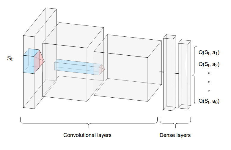
Figure 3: DQN architecture. (Created using NN-SVG and draw.io)
The state, which is an image of the screen, passes through a series of convolutional layers, where several filters, activations and pooling operations will be applied, to reduce it to a more manageable subspace. The output is then fed to a series of dense layers to compute the values of each of the actions, given the current state. The agent can then pick the next action using its policy (*), receive its reward, and perform the update to the $Q$ network using back propagation, with the aim of minimizing the MSBE function.
(*) a quick note on the different policies that can be used in practice:
-
Greedy policy: One of the simplest policies, similar to the one we have seen in the Q-Learning section, where the agent always chooses the action with the highest Q-value:
\[\pi^*(s)=arg\ max_a Q^*(s, a) \ \forall s \in S\]This policy lacks the property of exploration. In fact, it will keep exploiting the action that happened to be yielding good results at a certain point in time, but that may not necessarily be the optimal one, while ignoring other actions that may be better.
-
Epsilon-greedy policy: the agent takes action using the greedy policy with a probability of \(1−\epsilon\) and a random action with a probability of \(\epsilon\), where \(\epsilon\) is a real number close to zero ($0.1$ for example).
\[a_t = \begin{cases} arg\ max_a Q^*(s, a), & \mbox{with probability } 1-\epsilon \\ \text{a random action}, & \mbox{with probability } \epsilon \end{cases}\]Unlike the first one, this policy explores too much. In fact, even if the agent comes across the optimal action, this method keeps allocating a fixed percentage of time for exploration, thus missing opportunities to increase the total reward.
-
Decaying epsilon-greedy policy: the agent takes action using the epsilon-greedy policy, where \(\epsilon\) starts out with a high value, and thus a high exploration rate. Over time, \(\epsilon\) grows ever smaller until it fades out, hopefully as the policy has converged. This way, the optimal policy can be executed without having to take further, possibly sub optimal, exploratory actions.
As far as this implementation is concerned, the policy that has been used is the decaying epsilon-greedy policy, which \(\epsilon\) starting out at \(1\) and decaying over time with a multiplicative factor of \(0.996\).
To gain computational efficiency, we perform some pre-processing on the state before feeding it to the DQN. Typically, we get an RGB image from the emulator. We transform it to gray scale, and chop off some pixels on the left, right and the ground, since they are not involved in the action. We also crop the top of the image where the score is rendered, since we can keep track of it based on the reward the agent gets directly from the emulator.
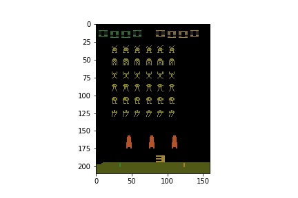
Figure 4: RGB image from the emulator.
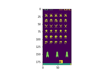
Figure 5: Pre-processed image to be fed to the DQN.
$\text{IV}$ - Results
Below are the curves of the scores obtained throughout the training phase by the DQN agent as well as a random agent used as a baseline:
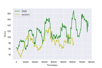
Figure 6: Scores obtained by the DQN during training, compared with those of a random agent as a baseline.
The DQN agent has played 100 episodes, 10000 time-steps each, and it has been able to improve its decision-making process as the training progresses. In fact, it starts by randomly selecting actions, waiting for the replay buffer to be sufficiently full to start the training. After several episodes of playing, the agent starts showing learning improvements and rather satisfactory results by the end of the training. This is due to the fact that its policy becomes progressively less random, as the update rule encourages it to exploit actions with higher rewards.
Here is a game where the agent is playing after being trained:
Figure 7: DQN agent playing Space Invaders after being trained for 100 episodes.
$\text{V}$ - Conclusion
The agent has done a pretty good job overall. Nevertheless, it has to be trained more and perhaps playing around with different hyper-parameters as well as the DQN’s architecture so that it can get a higher score. The source code of this post is available on my Github repository.
There is also one thing we can add in the pre-processing of the state to improve the performance. Since we are feeding one frame at a time to the DQN, the agent does not get a sense of motion and will have no idea which way the aliens are moving. This highly compromises the way actions are chosen. One way to solve this problem is to change the state we give to the agent. Instead of giving it just one single image at a time, we can stack $k$ successive frames on top of each other, forming a tensor of shape $(k, 210, 160, 3)$, that will represent our new state ready to be fed to the agent after being pre-processed as before.
$\text{VI}$ - Resources and further reading
[1] Playing Atari with Deep Reinforcement Learning
[2] Frame Skipping and Pre-Processing for Deep Q-Networks on Atari 2600 Games
[3] How RL agents learn to play Atari games