Generative Adversarial Networks For Outlier Detection

Introduction

The problem we are going to address in this post is that of outlier detection, which is the identification of observations that raise suspicions by differing significantly from the majority of the ordinary data. Applications are countless: from fraud detection, to health monitoring or intrusion detection.

Traditionally, the outlier detection problem is seen as supervised learning problem; a binary classification issue where we train a classifier to learn a boundary between the two classes; normal data and outliers. But these types of discriminative models tend to perform poorly, mainly due to the problem of unbalanced data. In fact, outliers, due to their rarity, generally represent a rather small percentage compared to the normal data. This lack of balance between the classes largely compromises the learning. There are several solutions to address this problem such as oversampling or under-sampling of the data before the training but we are not going to address them because they are used in a supervised learning schema. The main reason why we are not interested in the supervised learning schema is to avoid the labor of manually labeling the training data. As we will see later in this post, using a generative adversarial model will help us automate this tedious task.

The remainder of this post will be organized as follows:

Generative Adversarial Networks’ architecture.
The mathematics behind Generative Adversarial Networks.
Framing the outlier detection problem.
Implementation.
Results
References and further reading

Without further ado, let’s get started.

Generative Adversarial Networks’ architecture

In machine learning, two kinds of models exist; generative models and discriminative models. Given a data set of samples and their corresponding labels $(X, y)$, a discriminative model will learn the boundary between the different labels; the conditional probability $P(y|X)$, while a generative model will learn the probability distribution that generates a samples of a given class $y$, $P(X|y)$.

Generative Adversarial Networks (GANs) are a type of neural networks belonging to the class of generative models, as their name implies. They consist of two communicating neural networks: a generator and a discriminator. The generator takes as input a noise and returns a generated sample, while the discriminator’s job is to learn the boundary between generated samples and real samples. Since GAN learn the probability distribution underlying the training data, we can then use them to generate a data point that does not necessarily belong to the training data but it is part of the range of possibilities and thus it can be a novel data point.

This neural networks’ architecture, that was proposed back in 2014 by Ian GoodFellow and others from the University of Montreal, has become the go-to when it comes to image generation, video generation and speech synthesis. But that is not an exhaustive list of its applications. In fact, several attempts have also been made to solve problems regarding outlier detection. One of them is the Single-Objective Generative Adversarial Active Learning (SO-GAAL) model that was proposed in 2019, and which we are going to address in this post. As the code that was originally proposed by the authors of the later paper was written using Keras, with TensorFlow as the backend engine, I decided to re-implement it using PyTorch, so that will be another added value of this post, as I have not found any PyTorch implementations at the time of writing the present post.

The figure below depicts the GAN architecture:

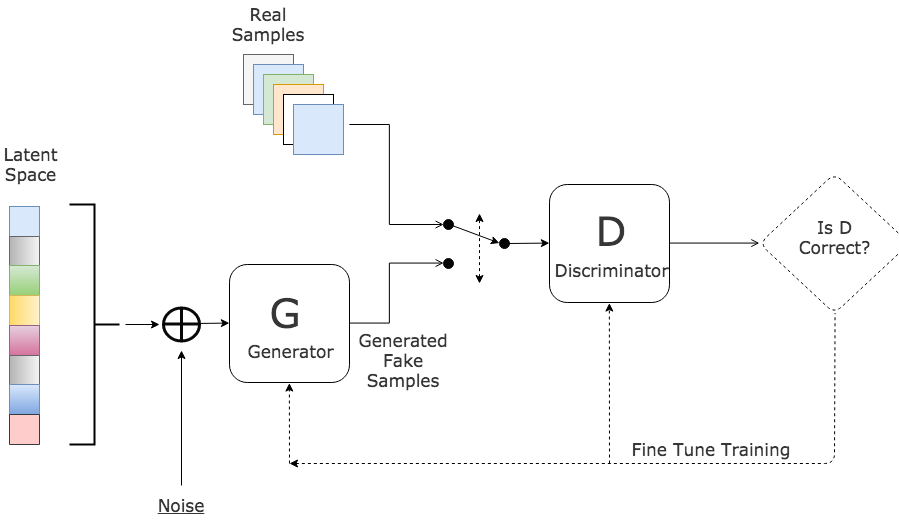
Figure 1: GAN's architecture. Source Link

We start by inputing some random numbers into the generator network. The later applies a series of matrix multiplication to output a fake sample. The discriminator’s job is to take a sample, either real or generated, and output a probability on whether this given sample is real or fake. Concretely, the generator trains itself in order for the samples it generates to pass the discriminator’s test; i.e. get the discriminator to classify fake samples as real. Whereas the discriminator trains itself in order to differ genuine from fake data. Both networks get better at their jobs as training progresses, until we finally have a generator that has become a master in faking and a discriminator that has become a master in noticing the nuance.

The mathematics behind GANs

For mathematics nerds that are out there, this section is for you. If you are not interested in the mathematics behind GAN and want to jump right into the code, then skip to the next section.

As you may already know, neural networks are optimized using an incremental process called gradient descent. Once the network has performed a forward-propagation, an output is returned, and is used to calculate the cost, defined as the difference between the network’s prediction and the desired output.

The cost functions of both the discriminator $D$ and the generator $G$ are derived from the cross-entropy loss function defined as:

\[L(\hat y, y) = y\space log(\hat y) + (1-y)\space log(1-\hat y)\]

where

\[- \space \hat y: \space \text{is the predicted probabilities}. \\ - \space y: \space \text{is the true label}.\]

Let’s start with the discriminator parameterized by $\theta_D$. If it is doing a good job, then for each sample $X$ drawn from the real data, it must output a probability $\hat y = D(X)$ that is close to $y = 0$, whereas for each noise $z$ given as input to the generator, it must output a probability $\hat y = D(G(z))$ that is close to $y = 1$, because it is a fake sample. Thus, we can write:

\[L(D(X), 0) = log(1-D(X))\] \[L(D(G(z)), 1) = log(D(G(z)))\]

These two quantities; equations (3) and (4), must be maximized in order for the discriminator to triumph. We can combine both of them in one expression, which is called the discriminator’s cost function:

\[L_D(x, G; \theta_D) = log(1-D(x)) + log(D(G(z)))\]

Meaning that the discriminator’s objective is to find the best parameters $\theta_D$ that maximizes its cost function. Thus the discriminator’s optimization problem can be written as:

\[\underset{\theta_D}{max}\space L_D(x, G; \theta_D)\]

Now let’s focus on the generator parameterized by $\theta_G$. The generator’s job is to fool the discriminator, meaning that it has to get the later to classify each fake sample $G(z)$ as not fake; $y= 0$. Thus we can write its cost function as follows:

\[L_G(z, D; \theta_G) = L(D(G(z)), 0) = log(1-D(G(z)))\]

Meaning that the generator’s objective is to find the best parameters $\theta_{G}$ that maximizes its cost function, thus its optimization problem can be written as:

\[\underset{\theta_G}{max}\space L_G(z, D; \theta_G)\]

Let’s stop for a second and try to analyze the relationship between the two cost functions $L_D$ and $L_G$.

Below is the plot of two functions; $log(x)$ and $log(1-x)$, in the interval $[0, 1]$.

Figure 2: Log function plot

We can see that, in the interval $[0, 1]$, maximizing $log(1-x)$ is the same as minimizing $log(x)$. Thus the generator’s optimization problem can be rewritten as follows:

\[\underset{\theta_G}{min}\space [log(D(G(z)))]\]

Which is equivalent to:

\[\underset{\theta_G}{min}\space L_D(x, G; \theta_D)\]

This means that the generator is trying to minimize what the discriminator is trying to maximize (*). This is called a zero-sum game (if one gains, another loses), and it is what motivates both of the networks to improve their functionalities as the training progresses.

(*) A little clarification on this point: even if the discriminator’s cost function has one more term than the generator’s cost function, we said that the function being optimized is the same, how come ? The additional term $log(1-D(x))$ that is present in $L_{D}$ does not depend on the generator’s parameters $\theta_G$, and thus it can safely be added to the generator’s optimization problem as a constant with respect to $\theta_G$ that won’t affect the final results.

Framing the outlier detection problem

We are going to approach outlier detection as a binary-classification issue using the SO-GAAL model stated in the introduction. The idea behind this model is that we are going to use a GAN that can directly generate informative potential outliers based on the game between the generator and the discriminator. More specifically, we are going to suppose that the distribution generating the normal data is not the same as the distribution generating the outliers. This way, we are going to use the generator to create potential outliers that are going to be added to the initial dataset progressively to better train the discriminator (the classifier we are interested in). As the training progresses, hopefully, the generator will become expert at generating potential outliers that look like the real data, and the discriminator will become expert at noticing the nuance. Additionally, by the end of training, we throw away the generator whose job was only to help us train the discriminator that we are going to keep.

This approach saves us mainly from the problem of unbalanced data that we generally encounter in outlier detection problems. In fact, the percentage of outliers in a dataset is generally very low compared to the normal data, which makes the dataset unbalanced and thus compromises the learning. With this approach, we are making sure to balance between normal data and the generated outliers before training the model, while avoiding the tedious task of manually labeling the data.

Implementation

As it has been mentioned in the introduction, we are going to train a SO-GAAL model for outlier detection. As an added value of this post, I have decided to implement it using PyTorch, as the original implementation was in Keras with TensorFlow as the backend engine, and at the time of writing this post, I have not found any available PyTorch implementations.

The implementation process will be as follows:

Importing modules and retrieving hyper-parameters from the command line.
Preparing the data (Extract Transform Load).
Building the model.
Training the model.
Analyzing the results.

1. Imports and hyper-parameters’ retrieval from the command line

import math
import matplotlib.pyplot as plt
import numpy as np
import pandas as pd
from collections import defaultdict # to store the training history
import argparse # to parse command line arguments

# PyTorch modules
import torch
import torch.optim as optim # For the optimizer
import torch.nn as nn # For the network's layers
import torch.nn.functional as F # For the loss function

def parse_args():
    """
    parsing the hyperparams specified in the command line
    """
    parser = argparse.ArgumentParser(description="Run SO-GAAL.")
    parser.add_argument('--path', nargs='?', default='Data/Annthyroid',
                        help='Input data path.')
    parser.add_argument('--stop_epochs', type=int, default=20,
                        help='Stop training generator after stop_epochs.')
    parser.add_argument('--lr_d', type=float, default=0.01,
                        help='Learning rate of discriminator.')
    parser.add_argument('--lr_g', type=float, default=0.0001,
                        help='Learning rate of generator.')
    parser.add_argument('--decay', type=float, default=1e-6,
                        help='Decay.')
    parser.add_argument('--momentum', type=float, default=0.9,
                        help='Momentum.')
    return parser.parse_args()

args = parse_args()

2. Preparing the data (Extract Transform Load)

In this phase, we have first to Extract the dataset from the source. In our case, we are going to use onecluster dataset that is available in the GAAL original github repository. This dataset contains 1000 data points, 2% of which are outliers.

def load_data():
    # get the data from file
    data = pd.read_table('{path}'.format(path=args.path), sep=',', header=None)
    # shuffle the data
    data = data.sample(frac=1).reset_index(drop=True)
    # retrieve indices and labels 
    id = data.pop(0)
    y = data.pop(1)
    # prepare features and target
    data_x = data.values
    data_id = id.values
    data_y = y.values
    
    return data_x, data_y, data_id

data_x, data_y, data_id = load_data()

This is how our dataset looks like:

id	label	x	y
0	nor	0.572606	0.445607
1	nor	0.426427	0.442882
2	nor	0.527975	0.556830
3	nor	0.504129	0.476744
4	nor	0.443147	0.485990

And here is a plot of all the data points:

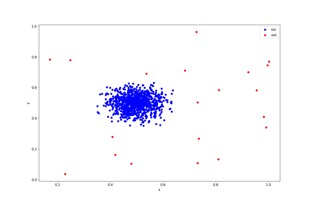
Figure 3: Onecluster dataset plot

# map existing labels to integers
data_y[data_y == 'nor'] = 1
data_y[data_y == 'out'] = 0
data_y = data_y.astype(np.int32)

Then we have to Transform the data to a tensor form in order for PyTorch to interpret it. Since we have numpyarrays output from the previous phase, we will make use of torch.utils.data.TensorDataset to transform the data to a tensor set:

# create tensors from np arrays
data_x_tensor = torch.Tensor(data_x)
data_y_tensor = torch.Tensor(data_y)

# Create a tensor dataset
train_set = torch.utils.data.TensorDataset(data_x_tensor, data_y_tensor)

And finally, we have to Load the data into an object to make it easily accessible. For this torch.utils.data.DataLoader is our go to:

# Specify a batch size to split the training set into
# the batch size will have a minimum value of 500
data_size = data_x.shape[0]
batch_size = min(500, data_size)
# Create a train loader
train_loader = torch.utils.data.DataLoader(train_set, 
                                           batch_size=batch_size,
                                           shuffle=True,
                                           drop_last=True)

The DataLoader combines a dataset and a sampler, and provides an iterable over the given dataset. Concretely, it shuffles the given dataset before it splits it into several batches of size batch_size over which we are going to iterate in the training phase. We drop the last batch just in case it is incomplete.

3. Building the model

As discussed earlier, the model will consist of two communicating networks; the discriminator and the generator. As you may already know, every neural network in PyTorch must inherit torch.nn.Module; the base class for all neural network modules, and it must also override the forward() method. I have added a method that will be applied recursively on the network to initialize the weights its layers.

# Generator
class Generator(nn.Module):
    def __init__(self, latent_size):
        super().__init__()
        self.model = nn.Sequential(
            nn.Linear(latent_size, latent_size),
            nn.ReLU(),
            nn.Linear(latent_size, latent_size),
            nn.ReLU()
        )
        # initialize the weights
        self.model.apply(self._identity_init)

        # checkpoint dir to save and load the model
        self.checkpoint_dir = './chkpt/generator/'

    def forward(self, input):
        return self.model(input)

    def _identity_init(self, m):
        if type(m) == nn.Linear:
            nn.init.eye_(m.weight)
            m.bias.data.fill_(1)

# Discriminator
class Discriminator(nn.Module):
    def __init__(self, latent_size, data_size):
        super().__init__()
        self.model = nn.Sequential(
            nn.Linear(latent_size, math.ceil(math.sqrt(data_size))),
            nn.ReLU(),
            nn.Linear(math.ceil(math.sqrt(data_size)), 1),
            nn.Sigmoid()
        )
        # initiliaze the weights
        self.model.apply(self._xavier_init)

        # checkpoint dir to save and load the model
        self.checkpoint_dir = './chkpt/discriminator/'

    def forward(self, input):
        return self.model(input)

    def _xavier_init(self, m):
        if type(m) == nn.Linear:
            nn.init.xavier_normal_(m.weight)
            m.bias.data.fill_(0.05)

print(Discriminator(10, 120))
print(Generator(10))

Discriminator(
  (model): Sequential(
    (0): Linear(in_features=10, out_features=11, bias=True)
    (1): ReLU()
    (2): Linear(in_features=11, out_features=1, bias=True)
    (3): Sigmoid()
  )
)
Generator(
  (model): Sequential(
    (0): Linear(in_features=10, out_features=10, bias=True)
    (1): ReLU()
    (2): Linear(in_features=10, out_features=10, bias=True)
    (3): ReLU()
  )
)

Both $D$ and $G$ are two-layer networks. All the layers are activated using ReLU function, except the last layer of $D$ that squashes the output into a range of $[0, 1]$ using the sigmoid activation function to make it capable of predicting a probability. As far as the other hyper-parameters are concerned, such as the layers’ dimensions, I have kept the same ones as those that were originally proposed by the authors of the GAAL paper in their original Keras implementation.

4. Training the model

Now that the model is built, it is time for training. Below are the steps we are going to follow:

We instantiate the model; i.e. the discriminator and the generator as well as their optimizers and loss functions.
We get a batch from the training set, in our case we are going to use the train_loaderthat contains all the batches, and we get the generator to create a fake sample as well.
We pass the batch through the networks in order to get predictions.
We compute the loss for each network using the loss function we have specified in step 1.
We compute the gradient of the loss function with respect to the network’s weights.
We update the weights using the gradients to reduce the loss using the optimizer specified in step 1.
We repeat steps 2-6 until one epoch is completed. An EPOCH being a complete pass through all the batches of the training set.
We repeat steps 2-7 for as many epochs required to obtain the desired level of accuracy.

The code below is the implementation of these 8 steps. I made sure to document each line so that you don’t get lost:

# create discriminator
discriminator = Discriminator(latent_size, data_size)
discriminator_optim = optim.SGD(discriminator.parameters(), lr=args.lr_d, dampening=args.decay, momentum=args.momentum)
discriminator_criterion = F.binary_cross_entropy
print(discriminator)

# Create generator
generator = Generator(latent_size)
generator_optim = optim.SGD(generator.parameters(), lr=args.lr_g, dampening=args.decay, momentum=args.momentum)
generator_criterion = F.binary_cross_entropy
print(generator)

# Start training epochs
for epoch in range(epochs):
    
    # go over batches of data in the train_loader
    for i, data in enumerate(train_loader):

        # Generate noise
        noise_size = batch_size
        noise = np.random.uniform(0, 1, (int(noise_size), latent_size))
        noise = torch.tensor(noise, dtype=torch.float32)

        # Get training data
        data_batch, _ = data

        # Generate potential outliers
        generated_data = generator(noise)

        # Concatenate real data to generated data
        X = torch.cat((data_batch, generated_data))
        Y = torch.tensor(np.array([1] * batch_size + [0] * int(noise_size)), dtype=torch.float32).unsqueeze(dim=1)

        # Train discriminator
        # enable training mode
        discriminator.train()
        # getting the prediction
        discriminator_pred = discriminator(X)
        # compute the loss
        discriminator_loss = discriminator_criterion(discriminator_pred, Y)
        # reset the gradients to avoid gradients accumulation
        discriminator_optim.zero_grad()
        # compute the gradients of loss w.r.t weights
        discriminator_loss.backward(retain_graph=True)
        # update the weights
        discriminator_optim.step()
        # Store the loss for later use
        train_history['discriminator_loss'].append(discriminator_loss.item())

        # Train generator
        # create fake labels
        trick = torch.tensor(np.array([1] * noise_size), dtype=torch.float32).unsqueeze(dim=1)
        # freeze the discriminator
        discriminator.eval()
        if stop == 0:
            # enable training mode for the generator
            generator.train()
            # compute the loss
            generator_loss = generator_criterion(discriminator(generated_data), trick)
            # reset the grads
            generator_optim.zero_grad()
            # compute the grads
            generator_loss.backward(retain_graph=True)
            # update the weights
            generator_optim.step()
            # store the loss
            train_history['generator_loss'].append(generator_loss.item())
        else:
            generator.eval()  # enable evaluation mode
            generator_loss = generator_criterion(discriminator(generated_data), trick)
            train_history['generator_loss'].append(generator_loss.item())

Results

The metric we are going to use to evaluate the results is the Area Under the Receiver Operating Characteristic (AUC-ROC).

The ROC curve provides a comprehensive view of the model performance at various thresholds settings by plotting the True Positive Rate and the False Positive Rate against each other.

The AUC statistic measures the entire two-dimensional area underneath the entire ROC curve, and thus provides an aggregate measure of performance across all possible classification thresholds. Higher the AUC better the model.

# Detection result for current epoch
# enable evaluation mode
discriminator.eval()
# computing probabilities
p_value = discriminator(data_x_tensor)
# create a dataframe of probabilities
p_value = pd.DataFrame(p_value.detach().numpy())
# create a dataframe of true labels
data_y = pd.DataFrame(data_y)
# create a result dataframe predicted probabilities/true labels
result = np.concatenate([p_value, data_y], axis=1)
result = pd.DataFrame(result, columns=['p', 'y'])
result = result.sort_values('p', ascending=True)

# Calculate the AUC
from sklearn import metrics
fpr, tpr, _ = metrics.roc_curve(result['y'].values, result['p'].values)
AUC = metrics.auc(fpr, tpr)

for _ in train_loader:
    train_history['auc'].append(AUC)

plot(train_history)

plot is a helper function that takes the training history and produce a summarized plot if the discriminator and generator respective losses as well as the AUC-ROC curve:

def plot(train_history):
    dy = train_history['discriminator_loss']
    gy = train_history['generator_loss']
    aucy = train_history['auc']
    x = np.linspace(1, len(dy), len(dy))

    plt.plot(x, dy, color='blue', label='Discriminator Loss')
    plt.plot(x, gy, color='red', label='Generator Loss')
    plt.plot(x, aucy, color='yellow', linewidth='3', label='ROC AUC')
    # plot the final value of AUC
    plt.axhline(y=aucy[-1], c='k', ls='--', label='AUC={}'.format(round(aucy[-1], 4)))

    plt.legend(loc='best')
    plt.show()

Figure 4: Learning curves on Onecluster dataset (generator's bias initialized to $1$)

Figure 5: Learning curves on Onecluster dataset (generator's bias initialized to $1e-5$)

Figures 4 and 5 represent the learning curves obtained after training with different initial values of the generator’s bias. On the left figure, we can see that the model has over-fit since both the discriminator’s training loss and the test AUC are very low. The generator’s loss increase can be explained by the fact that it is generating data points that are easy for the discriminator to spot as outliers. On the right figure, it is what we generally expect from a GAN after training. At the beginning, the discriminator’s loss is decreasing because the generator performs poorly. After the first 1000 epochs, the generator starts to fool the discriminator, which results in both losses changing their directions. After 2000 epochs of training, both networks begin to see their losses converging to a fixed value. The test AUC is pretty high as well, meaning that the discriminator did a good job when tested.

Below is the result that I was been able to reproduce from the original code proposed by the authors, available in the github repository mentioned in the references:

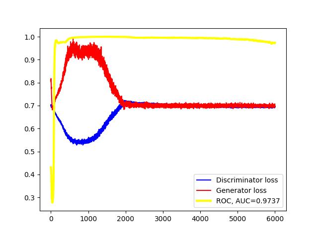
Figure 6: Original learning curves on Onecluster dataset

The learning curves as well as the test AUC are pretty close to those we have obtained in Figure 5. The slight differences between them may be due to implementation differences between Keras and PyTorch in some functions, mainly in the initialization methods, as well as the different seeds used to initialize the weights.

Conclusion

Thank you for making it this far. In this post we addressed the SO-GAAL model to solve the problem of outlier detection. As we have seen, SO-GAAL is a GAN that directly generates informative potential outliers to assist the classifier in describing a boundary that can separate outliers from normal data effectively. We have tested this model on the Onecluster dataset; a synthetic and highly unbalanced dataset. The obtained results are pretty satisfactory, nevertheless, the model has to be tested on real datasets. You can download the complete code (link in the references) and play around with it. As an improvement of the code, there are several features that can be added. First, we can build a run manager to experiment with other hyper-parameters for tuning purposes. Second, we can add TensorBoard support to further track the model’s performance. And finally, training GANs is very time-consuming, especially on modest hardware. For this reason, we can add GPU support to the code to accelerate the learning, since PyTorch allows us to do so easily.