Genetic Algorithms

Introduction

I have called this principle, by which each slight variation, if useful, is preserved, by the term Natural Selection.

Charles Darwin $-$ The Origin of Species

In 1859, the English naturalist Charles Darwin put forth his now Theory of Evolution in a book entitled “On the Origin of Species”. It is one of the most influential books in the human history because it has drastically shifted our perception of the world and our view of biology and biological systems.

Since Mother Nature has always been a great source of inspiration and fascination, Genetic Algorithms (GAs) are a family of optimization techniques that are “bio-inspired”. They mimic the biological processes of reproduction, natural selection and the survival of the fittest, to find the true or approximate solution for a given optimization problem. The idea behind them is simple yet so powerful. The search for the “fittest” candidate happens in generations. First, we start with a random population of individuals. Then, we set a criterion by which individuals from the current generation will be selected. Once selected, these individuals are invited to pass on their genes to the next generation by means of reproduction. We keep on going with this process until a maximum number of generations has been reached or a satisfactory enough solution has been found.

By the end of this article, you will be able to understand the basic concepts and terminology used in Genetic Algorithms. You will also be able to implement, from scratch, a Genetic Algorithm in Python and see it working in action on a dummy problem. Principles like “population”, “fitness”, “mutation”, “crossover” and “selection” will no longer be a mystery to you.

The remainder of this article will be organized as follows:

Background.
Genetic Algorithms in action: Evolving a “Hello World” sentence.
Conclusion.
References and further reading.

Background

Genetic Algorithms (GAs) were first described by John Henry Holland in the 1960s at the University of Michigan and were further developed by him and his students and colleagues, leading to the publication in 1975 of his book called “Adaption in Natural and Artificial Systems”. John Koza, one of Holland’s students, made the first commercial use of this family of methods by co-founding Scientific Games Corporation; which is an American corporation that provides gambling products and services to lottery and gambling organizations.

In 2006, NASA developed what’s called an evolved antenna, based on a GA, for its Space Technology 5 (ST5) mission. It is an X-band antenna whose shape was evolved starting from simple shapes and by getting some of its elements modified semi-randomly each time. The final result was a shape that has never been used before and were much more effective than the previously used ones.

Before diving into the implementation of the genetic algorithm, it is necessary to go through some basic terminology that will be used throughout this article as well as in the coding section. First things first, an individual is a possible solution to the optimization problem at hand. It takes part of a population, which is the group of all individuals. Each individual of the population thrive to survive by being the fittest individual; i.e. the optimal solution to the fitness function, which is the function we are optimizing. Finally, a score assigned to each individual of the population assessing how good or bad it is at solving the fitness function. This score is called the fitness score.

Below is the overall flowchart of a genetic algorithm:

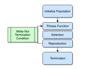
Figure 1: Genetic Algorithms Flowchart

Since genetic algorithms are a large family of algorithms, they differ based on the problem at hand but all share the common structure, depicted above. The algorithm starts by randomly initializing a population of individuals. Each individual of the population is evaluated by computing its fitness score using the fitness function. Then, a subset of the population is probabilistically selected based on the fitness scores. This subset of individuals, also called the fittest individuals, are invited to pass on their genes to the next generation by means of reproduction. And the process starts over again with a newly created generation and keeps going until we run out of budget or have found a satisfactory enough solution.

In the next section, I am going to delve into the details of each step, in the light of a practical example, including the corresponding implementation of each step in Python.

Genetic Algorithms in action: Evolving a “Hello World” sentence.

Now that you have an idea about the fundamental structure of Genetic Algorithms, let’s build a genetic algorithm that will generate a target sentence that we will specify. Let’s say the famous “Hello World”. As you will see, the algorithm starts by randomly generating multiple sentences. You will also see that the generated sentences get better and better and the overall score of the population gets higher and higher as the learning progresses.

First, let’s import the necessary packages and fix a seed for reproducibility.

# A system that uses a genetic algorithm to generate a target sentence
import random
import matplotlib.pyplot as plt
import numpy as np
import string

# fixing the seed of reproducibility
seed = 123
np.random.seed(seed)
random.seed(seed)

As depicted in the flowchart of Figure 1, there are five main steps to implement a genetic algorithm. The first one is initializing the population.

1. Initializing the population

As a starting point, the process begins with a set of individuals called population; which are potential solutions to the problem at hand. Each individual has a set of components that defines it. The number of components depends on the size of the search space. In our case, we want the algorithm to generate a target sentence of length 11. Thus, the search space is 11-dimensional. This implies that each individual will be represented as an 11-dimensional vector, and each component of this vector will defined in the set of alphabetic and special characters, as depicted in the example below :

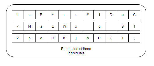
Figure 2: Example of a population of individuals.

Let’s build a class that will represent our genetic algorithm, with a method that initializes the population:

class GeneticAlgorithm:
    def __init__(self,
                 fitness_function,
                 num_attributes=2,
                 population_size=100,
                 crossover_prob=.75,
                 mutation_prob=.05):
        self.fitness_function = fitness_function
        self.num_attributes = num_attributes
        self.population_size = population_size

        self.crossover_prob = crossover_prob
        self.mutation_prob = mutation_prob

        self.population = None
        self.population_avg_score = 0
        self.fitness_scores = None
        self.fittest_individuals = None

    def initialize_population(self):
        """
        init a population of individuals
        args:
            num_attributes: length of each individual (attributes)
            population_size: number of individuals
        returns:
            population_size lists of n length each.
        """
        attributes = []

        for attribute in range(self.num_attributes):
            attributes.append(
                np.random.choice(
                    list(string.punctuation + string.ascii_letters +
                         string.whitespace),
                    size=self.population_size))

        self.population = np.array(attributes).T

Now that we have our population, we have to evaluate each individual in the pool. This is where the fitness function comes into play.

2. Fitness function

The fitness function is the term that designate the criterion upon which individuals are evaluated. It is a way to quantify the goodness or badness; i.e fitness, of each individual vis-à-vis the problem at hand. This quantification is called the fitness score, and it is associated with each individual. It helps the algorithm decide which individuals to keep and which individuals to toss over the course of generations.

Back to our example, the fitness function will be defined as the number of characters that the genetic algorithm has got right compared with the target sentence.

def fitness_function(individual, target_sentence='Hello World'):
    """
    computes the score of the individual based on its performance
    approaching the target sentence.
    """

    assert len(target_sentence) == len(individual)

    score = np.sum([
        individual[i] == target_sentence[i]
        for i in range(len(target_sentence))
    ])
    return score

And let’s add a method to the Genetic Algorithm class to compute the fitness score of each individual in the population.

class GeneticAlgorithm:
    def __init__(self,
                 fitness_function,
                 num_attributes=2,
                 population_size=100,
                 crossover_prob=.75,
                 mutation_prob=.05):
        self.fitness_function = fitness_function
        self.num_attributes = num_attributes
        self.population_size = population_size

        self.crossover_prob = crossover_prob
        self.mutation_prob = mutation_prob

        self.population = None
        self.population_avg_score = 0
        self.fitness_scores = None
        self.fittest_individuals = None

	# ... initialize_population

    def compute_fitness_score(self):
        """
        computing the fitness score of the population.
        args:
            individual: numpy array representing the chromosomes of the parent.
        returns:
            population_size lists of n length each.

        """
        scores = np.array([
            self.fitness_function(individual) for individual in self.population
        ])
        self.fitness_scores = scores

Once the fitness scores are computed, it is time for selection.

3. Selection

Selection is the process of choosing the fittest individuals within the initial population based on their fitness score. The main purpose of this phase is to choose the individuals whose offspring hence produced will have higher fitness scores. What we have to keep in mind during this phase is that the process of selection must be balanced. A very strong selection process will lead to the fittest individuals taking over the population, reducing the diversity and variation needed for exploration. On the other hand, a very weak selection process may lead to a very slow evolution.

There are several methods that can be used to select the best individuals within a population. We are going to implement the most commonly used one, which is the Fitness Proportionate Selection also known as the Roulette Wheel Selection.

Roulette Wheel Selection

In this method, a probability of selection is assigned to each individual within the population of interest. This probability is computed based on the fitness score of the individual at hand as well as the fitness scores of other individuals in the population. More specifically,

\[P(i)=\frac{fitness\_score(i)}{\sum_{j=1}^{N}{fitness\_score(j)}}\]

where $P(i)$ is the probability of selecting individual $i$, and $N$ is the population size.

class GeneticAlgorithm:
    def __init__(self,
                 fitness_function,
                 num_attributes=2,
                 population_size=100,
                 crossover_prob=.75,
                 mutation_prob=.05):
        self.fitness_function = fitness_function
        self.num_attributes = num_attributes
        self.population_size = population_size

        self.crossover_prob = crossover_prob
        self.mutation_prob = mutation_prob

        self.population = None
        self.population_avg_score = 0
        self.fitness_scores = None
        self.fittest_individuals = None

    # ... initialize_population

    # ... compute_fitness_score:

    def roulette_wheel_selection(self):
        """
        Select the fittest individuals based on their fitness scores.
        each individual is associated with its index in the input array.
        ---
        Args:
            fitness_scores: numpy array of fitness score of each individual
        Returns:
            parents:  
        """
        sum_scores = np.sum(np.abs(self.fitness_scores))
        selection_prob = np.abs(self.fitness_scores) / sum_scores

        parents = random.choices(self.population, weights=selection_prob, k=2)

        return parents

4. Reproduction

Now that we have selected the fittest individuals (parents), it is time to start populating the next generation. In this phase, there are two main operations that are performed on the selected individuals; crossover and mutation, as it is the case in sexual reproduction in the animal kingdom. When performing reproduction, we have to keep in mind that the size of the newly created generation must be the same as the size of the old one.

4.1 Crossover

Also called, recombination, this operation aims to combine genetic information of two parents to produce a new offspring. This recombination starts by selecting a random crossover point from within the genes of the parents. The information to the right of that point is swapped between the two parents resulting in two children carrying out genes from both parents, as illustrated below:

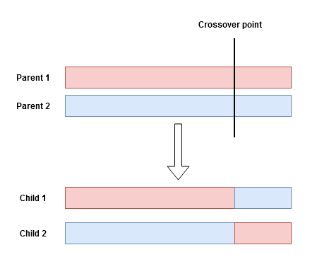
Figure 3: Illustration of a single-point crossover.

Depending on the size of the parents, we can set up more than one random crossover point, and each time the same operation took place. This is called Multi-Point Crossover.

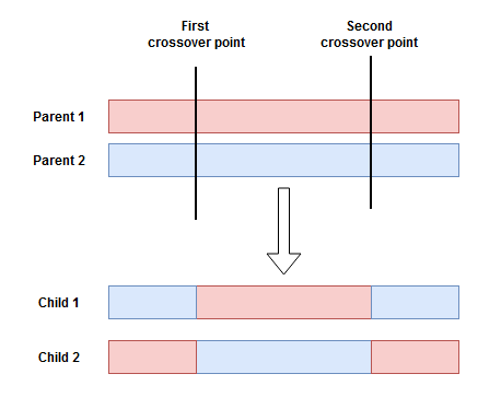
Figure 4: Illustration of a multi-point crossover.

4.2 Mutation

Similar to the one in the biological context, the mutation operator introduces diversity from one generation to another. It applies a small random tweak on the genes of an individual to get a new one, thus encouraging the algorithm to better explore the search space. These random tweaks on each gene of an individual are performed based on a mutation probability that has to be meticulously defined a-priori. In fact, when setting the mutation probability too high, too much information is lost, thus turning the algorithm into a random search within the search space.

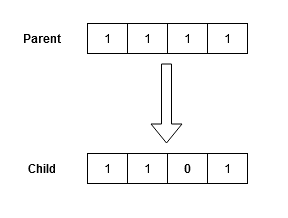
Figure 5: Illustration of a mutation.

Back to our use-case, let’s implement these two methods within our Genetic Algorithm class:

class GeneticAlgorithm:
    def __init__(self,
                 fitness_function,
                 num_attributes=2,
                 population_size=100,
                 crossover_prob=.75,
                 mutation_prob=.05):
        self.fitness_function = fitness_function
        self.num_attributes = num_attributes
        self.population_size = population_size

        self.crossover_prob = crossover_prob
        self.mutation_prob = mutation_prob

        self.population = None
        self.population_avg_score = 0
        self.fitness_scores = None
        self.fittest_individuals = None

    # ... initialize_population

    # ... compute_fitness_score

    # ... roulette_wheel_selection

    def run(self):
        """
        running the genetic algorithm to produce a new generation.
        """
        def cross_over(parents):
            """
            produces a new individual by combining the genetic information of both parents.
            Args:
                individual_1: numpy array representing the chromosomes of the first parent.
                individual_2: numpy array representing the chromosomes of the second parent.
            returns:
                child: newly created individual by cross over of the two parents.
            """
            if np.random.uniform() <= self.crossover_prob:
                parent_1, parent_2 = parents
                crossover_point = np.random.choice(
                    range(1, self.num_attributes))
                child = np.concatenate(
                    (parent_1[:crossover_point], parent_2[crossover_point:]))
                return child
            else:
                return random.choices(parents)[0]

        def mutate(individual):
            """
            produces a new individual by mutating the original one.
            Args:
                individual: numpy array representing the chromosomes of the parent.
            returns:
                new: newly mutated individual.
            """
            new_individual = []
            for attribute in individual:
                if np.random.uniform() <= self.mutation_prob:
                    new_individual.append(random.choice(string.ascii_letters))
                else:
                    new_individual.append(attribute)

            return new_individual

        new_population = []

        # reproduce the new population
        for _ in range(self.population_size):
            parents = self.roulette_wheel_selection()
            child = cross_over(parents)
            child = mutate(child)

            new_population.append(child)

        self.population = np.array(new_population)

5. Termination

In practice, we don’t want the GA to run ad infinitum. We set up a criterion that will indicate when the GA run will end. This can be one or a combination of the following termination conditions:

The algorithm has reached a pre-defined fitness value that is qualified as satisfactory.
The algorithm has reached a pre-defined number of generations.
The algorithm is no longer getting better results after a pre-defined number of successive runs.

In our case, we are going to set a pre-defined number of generations as well as a maximum number of successive runs without improvement.

def main():
    target_sentence = 'Hello World'
    np.random.seed(123)
    MAX_GEN = 100  # termination
    MAX_SUCCESS = 3  # termination
    NUM_ATTRIBUTES = len(target_sentence)
    POPULATION_SIZE = 500
    MUTATION_PROB = .01
    CROSSOVER_PROB = .75

    GA = GeneticAlgorithm(fitness_function,
                          num_attributes=NUM_ATTRIBUTES,
                          population_size=POPULATION_SIZE,
                          mutation_prob=MUTATION_PROB,
                          crossover_prob=CROSSOVER_PROB)
    GA.initialize_population()
    scores = []
    generation_counter = 0
    success_counter = 0

    while generation_counter < MAX_GEN and success_counter < MAX_SUCCESS:
        GA.compute_fitness_score()
        scores.append(np.mean(GA.fitness_scores))
        print('Generation', generation_counter, ", avg score:",
              scores[generation_counter], ", best:", GA.get_best())

        if GA.get_best() == target_sentence:
            success_counter += 1

        GA.run()
        generation_counter += 1

    plt.plot(scores)
    plt.xlabel('Generation')
    plt.ylabel('Average score per generation')
    plt.show()

main()

These are the results after running the program:

Generation 0 , avg score: 0.124 , best: Nwlsoo!,r/o
Generation 1 , avg score: 1.116 , best: Nwlsoo!,r/u
Generation 2 , avg score: 1.466 , best: Hwlsoo!,r/o
Generation 3 , avg score: 1.936 , best: NwlsokW,r/u
Generation 4 , avg score: 2.238 , best: Nwlso!Wr+u
Generation 5 , avg score: 2.602 , best: H&soo!,rld
Generation 6 , avg score: 2.886 , best: AwlsooWDrlH
Generation 7 , avg score: 3.174 , best: Adllo WDro	
Generation 8 , avg score: 3.436 , best: Hdllo WDroY
Generation 9 , avg score: 3.748 , best: Hdllo WDroY
Generation 10 , avg score: 4.094 , best: H	lsohWorld
Generation 11 , avg score: 4.356 , best: Hkl.o Wor/d
Generation 12 , avg score: 4.686 , best: Pelso WorlH
Generation 13 , avg score: 4.87 , best: Hwllo WDrlH
Generation 14 , avg score: 5.048 , best: Hwllo Whr/d
Generation 15 , avg score: 5.404 , best: Hwllo WDrld
Generation 16 , avg score: 5.586 , best: HellokWorlf
Generation 17 , avg score: 5.846 , best: Hwllo Worlo
Generation 18 , avg score: 6.082 , best: Hnllo World
Generation 19 , avg score: 6.242 , best: HUlso World
Generation 20 , avg score: 6.414 , best: Hello WDrld
Generation 21 , avg score: 6.604 , best: HJllo World
Generation 22 , avg score: 6.738 , best: Helso World
Generation 23 , avg score: 6.984 , best: Hello World
Generation 24 , avg score: 7.108 , best: Hello World
Generation 25 , avg score: 7.182 , best: Hello World
Generation 26 , avg score: 7.342 , best: Hello World
Generation 27 , avg score: 7.528 , best: Hello World
Generation 28 , avg score: 7.704 , best: Hello World

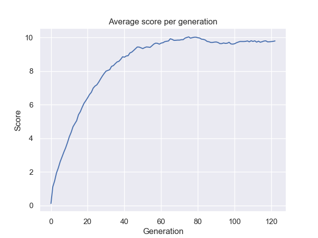
Figure 6: Average score per generation.

Starting with a population of $500$ individuals, the algorithm has evolved the target sentence in $23$ generations. From the above, it is shown that the average score of the population gets higher and higher, and the best individual of the population gets fitter and fitter. It is noteworthy that there are some parameters of the GA, in particular the population size and the mutation rate, governing the variance within the population. They are intimately linked to the overall performance of the algorithm. Let’s try to change some of these parameters and see how the system behaves.

Let’s fix the population size to $100$ and try different values of the mutation probability. Below is the evolution of the average score of each generation.

Figure 7: Average score per generation for several values of the mutation probability.

Figure 7 shows that the mutation probability is intimately linked to the performance of the algorithm. We see that the mutation probability of $0.01$ has evolved optimally, starting with a low score that gets higher over the course of generations. Whereas with the mutation probability of $1$, the GA has not evolved at all and with the mutation probability of $0$, the GA started evolving until plateauing around a score of $6$. As mentioned earlier, the mutation is used principally to introduce variance within the population. On one hand, setting it too high and the algorithm turns into a random search (valuable information is not preserved in the long run) thus the average score not evolving at all as shown by the green line in the plot above. On the other hand, setting the mutation probability to zero is not optimal either because the algorithm got stuck in a suboptimal solution and no longer evolves. The optimal way is to set the mutation probability to a value that introduces just enough variance to avoid getting stuck in a suboptimal solution while preserving valuable information in the long run from one generation to the other.

Now let’s fix the mutation probability to $0.01$ and change the population size:

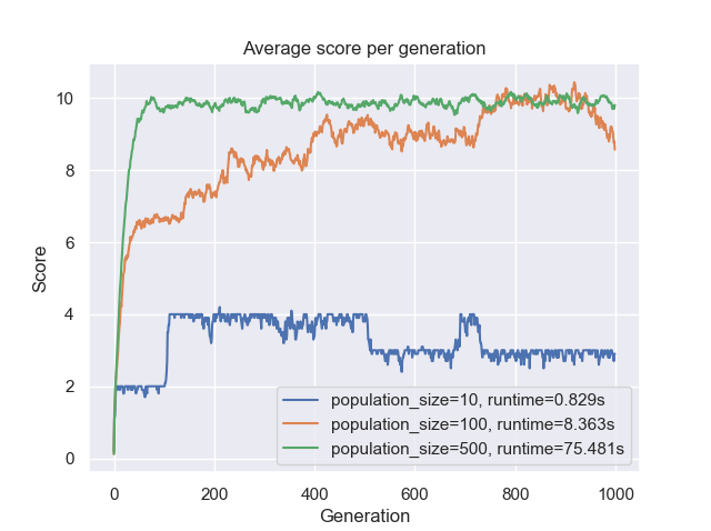
Figure 8: Average score per generation for several values of the population size.

Figure 8 shows two pieces of information. First, we see that the runtime is proportional to the population size. This is logical because the $10$ individuals require much less computation (smaller time complexity) than $500$. Second, we see that the higher the population size, the faster is the convergence point. The $500$ individuals converged in about $100$ generations whereas the $100$ individuals converged in about $700$ generations. This is due to the fact that with a bigger population, more variance is introduced. Thus the search space is explored more efficiently and therefore evolving much quickly towards the optimal solution.

Bottom-line is that there is a trade-off between variation and complexity. Having a large population size helps because we will have a larger pool to start with in terms of variation. But this comes at the cost of the algorithm taking forever to get to the optimal solution. With a smaller population size, the algorithm took much more generations to reach the optimal solution, but this happened quite faster in terms of runtime.

Conclusion

This was a short introduction to the broad field of Genetic Algorithms. I tried to keep it short and straight to the point. We have seen the fundamental terminology used in this field and implemented each step of the GA in Python. The full code is available on my GitHub. Feel free to clone the project and play around with the different hyper-parameters. You can also try to implement other sophisticated selection methods. And in the meantime, don’t forget to have fun..